Cancer Mortality Analysis
We used data from data.world called the OLS Regression Challenge, which were aggregated from the 2013 American Community Survey (census.gov), ClinicalTrials.gov, and Cancer.gov. The data contained the average cancer mortality across the United States between from 2010 through 2016. It also contains different demographic qualities such as income, ethnicity, education, average reported mortalities due to cancer, and birth rate to name a few.
Pre-processing
The original data set contained 3,047 observations representing the different counties in the United States along with 33 different demographic qualities. Since our project scope covers the states of California, South Carolina, and Illinois, these were filtered and integer encoded. This reduced our data to only 205 observations.
In addition, we:
removed
binnedincbecause median income per capita binned by decile is neither numeric nor factor.removed
pctsomecol18_24,pctemployed16_over,pctprivatecoveragealonebecause they contained lot ofNAvalues.extracted only State information from geography, where the original source contained County and State separated by comma.
Model Fitting
Since there were many variables, we used AIC and BIC to find the optimal model. We then searched for influential points for each model using Cook’s Distance and removed these from the set.
We used Fitted vs. Residual and Q-Q plot graphs to visually determine which model would be preferable. Based purely on the graphs, there’s no clear way to determine which would be better so we defer to quantitative testing by comparing their RMSE, adjusted R2, and results in of the Breusch-Pagan and Shapiro-Wilk Test.


In comparing the results, we find that most of the quantitative test results are the same. We did notice that the AIC model's $R^2$ was higher, which was expected for a model with more predictors. By comparing their Adjusted $R^2$ instead, we found a very small difference of 0.0073698.
Seeing as the models are very close, we opted to choose the BIC model as it had less predictors compared to the more complex AIC model. It turns out that these two models are actually nested, so we checked by running an ANOVA test. The test further confirmed that the smaller BIC model is preferred.

Prediction and Discussion
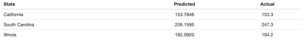
We predicted three observations from different states and we found that the model predicted very close to the actual target_deathrate. For the other observations, it was also fairly close. Thus, we think this model is very useful in predicting the Mean per capita (100,000) cancer mortality.
The observed data shows that counties with high median income and education has lower mean per capita (100,000) cancer mortality. It may be possible that cases with higher income can afford expensive treatments, thus reducing mortality rates compared to cases with less income. It is also possible to extrapolate that education might help lead good and healthy lifestyle.
From the coefficients we can infer that Mean per capita (100,000) cancer diagoses, Percent of county residents who identify as Black and Percent of county residents with employee-provided private health coverage has positive correlation with Mean per capita (100,000) cancer mortality.
Similarly, from the coefficients we can infer that Median Income and Percent of county residents ages 18-24 highest education attained (bachelor’s degree) has negative correlation with Mean per capita (100,000) cancer mortality.